On Time-varying Risk Premia

1Introduction

Most real-world allocation processes begin with a long-run equity premium estimate, often in the spirit of Ibbotson’s early work documenting historical equity, bond, and cash returns, and then ask whether today’s expected premiums should differ from that long-run average. That seemingly innocuous step is where confusion enters: long-run estimates are unconditional objects, while the risk-return tradeoff in asset-pricing models is inherently conditional. When investors observe factor “droughts” (value being the obvious example) or cyclical performance, the question is not whether time-varying premia can exist, but what that time variation means and how it should change implementation.

If you interpret all predictability as an anomaly, you will gravitate toward skepticism about factor investing. If you view predictability as compensation for state-dependent risk exposures and hedging demands, the right response is to model the conditioning information and understand which risks are being priced.

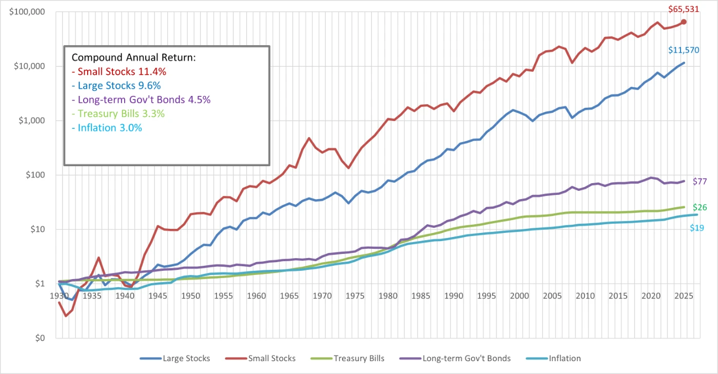
Figure 1 clarifies the core distinction that motivates this memo. The series provide an essential unconditional benchmark: long-run compounded premia are economically large, yet the realized path is highly nonuniform, with regime shifts that dominate investor experience at practical horizons. Classical pricing models reconcile these facts by treating expected returns as conditional: even if unconditional averages are stable, conditional betas and conditional prices of risk can move with the state, generating predictable variation in realized returns. The sections below show how CAPM rules out this mechanism by assumption, while CCAPM, ICAPM, and APT permit it in increasingly general ways.

2The Capital Asset Pricing Model

This is the classic Markowitz–Tobin setup that delivers the two-fund separation theorem: mean-variance investors are myopic and hold the market portfolio plus the risk-free asset. Expected excess returns line up on the security market line (SML),

(1)

and the slope of the SML is the market risk premium, . In the static CAPM, the market price of risk is constant, so predictably time-varying risk premia were interpreted as a pricing failure, i.e., an anomaly or market inefficiency, and motivated the large literature on conditional and intertemporal models.

3Conditional CAPM

The conditional CAPM of Hansen and Richard (1987) shares the core logic of the CAPM but allows for time variation in beta and the price of risk.

(2)

The subscript t denotes expectations conditional on the information set up to that period, hence the name, conditional CAPM. Investors are still myopic and the market portfolio remains mean-variance efficient, but at each point in time.

Not to be confused with the consumption CAPM of Breeden (1979), which carries the same abbreviation. We will save that for another day.

4Intertemporal CAPM

The intertemporal CAPM of Merton (1973) is a multi-period model where expected returns compensate for covariance with the market and with shocks to state variables that move the future investment opportunity set (hedging demands).

(3)

Here, the extra factors are returns on long-short portfolios (factors) that protect against shifts in, e.g., interest rates, volatility, or expected returns. The efficient portfolio is multi-dimensional; investors trade off current mean-variance and intertemporal hedging. The frontier is spanned by the market and the hedge portfolios tied to state variables. The slope becomes a vector of risk prices (, ).

These core insights have been extended in many directions, notably Campbell and Vuolteenaho (2004), which decomposes the market beta into cash-flow and discount-rate shocks, “bad” and “good” beta, where the former covaries with market downturns. Investors are willing to pay a premium for assets that hedge against bad times, but not for assets that covary with good times.

5Arbitrage Pricing Theory

The APT of Ross (1976) begins from the absence of arbitrage rather than a representative-investor optimization problem. If asset returns admit an approximate factor structure,

(4)

with idiosyncratic shocks that can be diversified away in large portfolios, then no-arbitrage implies the same linear restriction on expected excess returns as that found in equation (3), without requiring an explicit model of preferences, consumption, or the market portfolio. Furthermore, APT is agnostic about what the factors are: they may be macroeconomic shocks, statistical factors, or returns on traded factor-mimicking portfolios.

Time variation enters naturally through a conditional factor structure. Both factor loadings and prices of risk may vary with the information set at t, so that risk prices () can be forecast by state variables (e.g., term spreads, valuation ratios, volatility). This complements the practitioner tradition of measuring realized premia. In particular, the historical return series assembled by Ibbotson and Sinquefield (1979) makes clear that realized premia exhibit substantial variation across subperiods, a practical motivation for conditional specifications when translating historical averages into forward-looking expected returns.

Conclusion

Figure 1 highlights the practical source of confusion: long-run historical premia are economically large, yet realized performance varies sharply across subperiods and regimes. The static CAPM rules out state dependence by assumption, so predictable variation in expected excess returns is best interpreted as a failure of the model’s maintained assumptions rather than a refutation of risk premia. The conditional CAPM restores consistency by allowing both market betas and the market price of risk to move with the information set, while the intertemporal CAPM goes further by introducing additional priced sources of risk tied to shocks that shift the investment opportunity set and generate hedging demand. The APT reaches a similar linear pricing restriction from no-arbitrage without committing to a representative-agent structure, and it naturally accommodates time-varying risk prices through conditional factor models. The productive synthesis is to treat historical premia as long-run anchors, but to use conditional specifications and out-of-sample discipline when translating those averages into forward-looking expected returns and implementable portfolio decisions.

Back to research

References

- John Y. Campbell and Tuomo Vuolteenaho. “Bad Beta, Good Beta.” American Economic Review 94.5 (Dec. 2004), pp. 1249–1275.
- Lars Peter Hansen and Scott F. Richard. “The Role of Conditioning Information in Deducing Testable Restrictions Implied by Dynamic Asset Pricing Models.” Econometrica 55.3 (1987), pp. 587–613.
- Roger G. Ibbotson and Rex A. Sinquefield. “Stocks, Bonds, Bills and Inflation: Updates.” Financial Analysts Journal 35.4 (1979), pp. 40–44.
- Robert C. Merton. “An Intertemporal Capital Asset Pricing Model.” Econometrica 41.5 (Sept. 1973), p. 867.
- Stephen A. Ross. “The Arbitrage Theory of Capital Asset Pricing.” Journal of Economic Theory 13.3 (Dec. 1976), pp. 341–360.